Limitations of spike response model and coding
Review of Last Week’s Reading
Review of Last Week’s Reading
Keywords:
- Spiking train: a chain of action potentials (P3)
- Absolute refractory period: minimal distance between two spikes
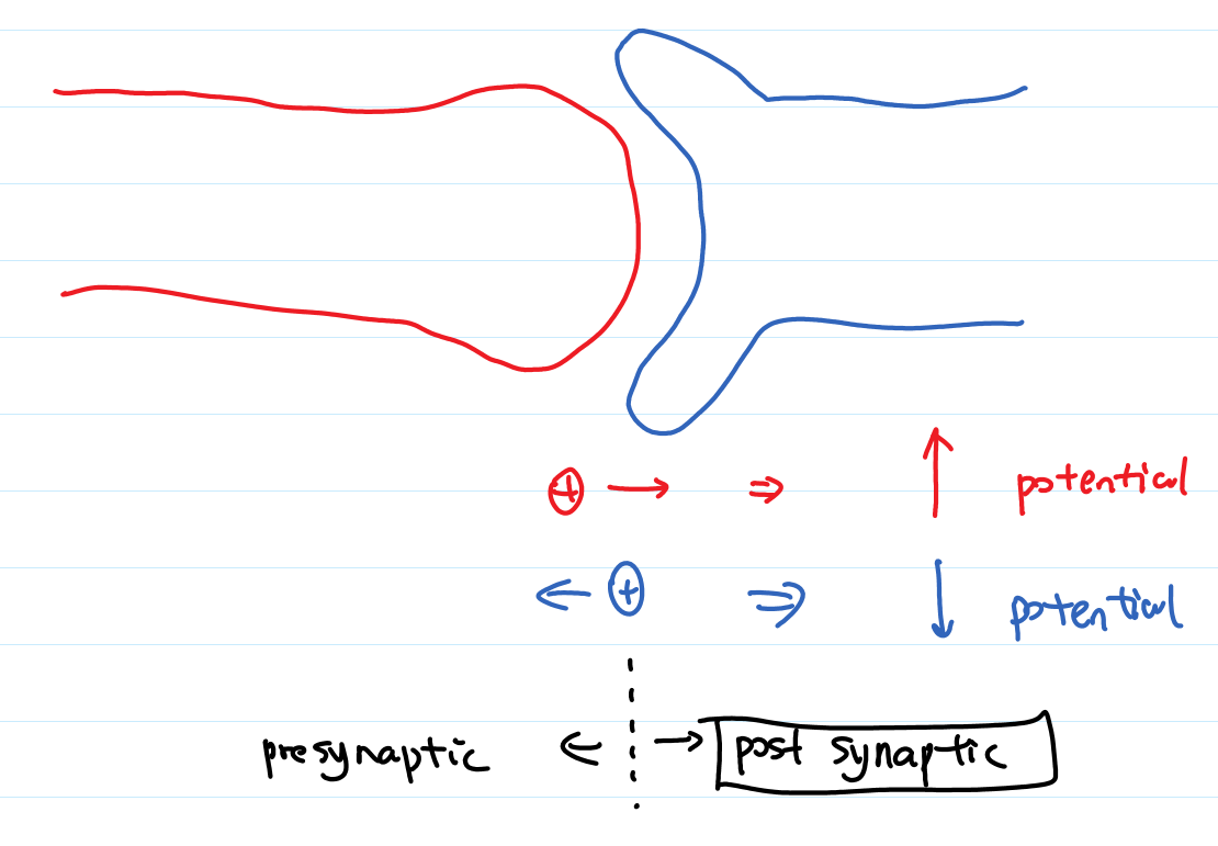
- synapses: chemical, electrical (gap junctions)
- excitatory and inhibitory: change of potential due to an arrival spike, positive-> excitatory, negative -> inhibitory
- postsynaptic potential: voltage response
- PSP: postsynaptic potential
- IPSP/EPSP: I-> Inhibitory, E->Excitatory
- depolarize/hyperpolarize: increase potential->depolarize, decrease potential->hyperpolarize
- $\text{SRM}_0$: Each response to the incoming spikes are linearly summed up until a spike is triggered. (P7, Equation 1.3)
- $$u_i=\eta(t-\hat t_i)+ \sum_j \sum_f \epsilon_{ij}(t-t_j^{(f)}) + u_{\mathrm{rest}} $$
- adaptation: fig1.5
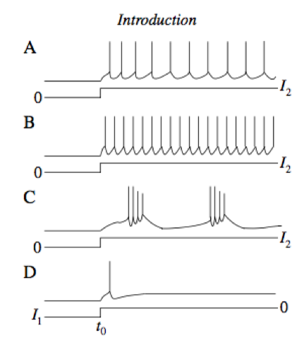
- regular firing neurons/fast-spiking neurons/bursting neurons: fig 1.3. fast-spiking is what would SRM0 give us
- rebound spikes: fig 1.3 D
Limitations (cont’d)
Saturating Excitation and Shunting Inhibition
Facts: shape of PSP depends on
- level of potential,
- internal state of the neuron, like state of ion channels.
- The PSP depends on the potential of the neuron itself when the presynaptic spike arrives.
 Interesting facts:
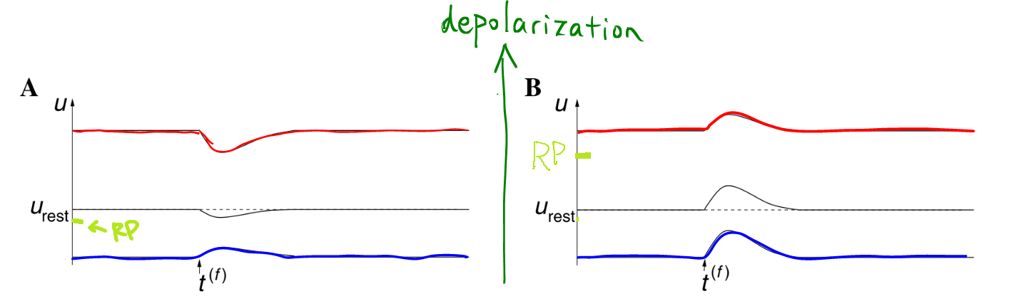
- IPSP, usually leads to hyperpolarization. Amplitude is larger if the neuron has a higher potential when presynaptic spike arrives. However, the response is reversed, i.e., depolarizing, if the potential is already hyperpolarized a lot. Reason for a reversal response is that PSC switch to the other direction if the potential $u_0$ before spike is due to the wrong direction of the PSC.
- EPSP is larger given lower potential, i.e., more depolarization.
- IPSP, usually leads to hyperpolarization. Amplitude is larger if the neuron has a higher potential when presynaptic spike arrives. However, the response is reversed, i.e., depolarizing, if the potential is already hyperpolarized a lot. Reason for a reversal response is that PSC switch to the other direction if the potential $u_0$ before spike is due to the wrong direction of the PSC.
- PSC: postsynaptic current, which is proportional to the actual effective potential (reversal potential) on the neuron membrane.
- Shunting inhibition: A few inhibitory synapses shunt input of a few hundred excitatory synapses.
Neuronal Coding
One of the ways to present neuron spikes is the spatio-temporal patterns of pulses. (Fig 1.8)
- mean firing rate: $\nu= \frac{n_{\mathrm{sp}}(T)}{T}$, i.e., number of spikes during time $T$ divided by the time span $T$.
- History:
- Adrian, 1926, 1928: firing rate of stretch receptor neurons -> forces on muscle
- Temporal average: is an approximation by filtering a lot of information out.
- Objections:
- brain activities are fast, too fast to allow coding in temporal average. 400ms for example.
- evidence of temporal correlations betwen pulses of different neurons.
- stimulus-dependent synchronization of activity in many neurons
Rate Codes
Mean firing rate:
-
temporal averaging (fig 1.9) (Boltzmann?):
- $\nu=\frac{\text{No. of spikes during time }T}{\text{time }T}$.
- Usually $T\sim 100\mathrm{ms}$ or $T\sim 500\mathrm{ms}$.
- The general principle is to increase the time until no change in the average during a single stimulus.
- Example: leech touch receptor,stronger the stimulus -> more spikes during a $500\mathrm{ms}$ average.
- Working if
- mapping of one input variable to a single output result, i.e., $\mathrm{single output}=f(\mathrm{single input})$. Example: force on receptors -> average firing rate.
- stimulus is not fast-varying
- doesn’t require fast reaction
- Evidence for other types of coding:
- Fly react in 30-40ms
- Human react to some visual in a $\sim 10^2$ms
- Human can detect images even the images was shown for 14-100ms.
-
averaging over repetitions of experiments (fig 1.10) (partial ensemble average, Gibbs?):
- many runs of experiment + PSTH (fig 1.10)
- PSTH: peri-stimulus-time histogram, peri means we count the spikes in a time interval $\Delta t$.
- Spike density: $\rho(t) = \frac{n_K(\text{from } t \text{ to }t+\Delta t)}{K}/\Delta t$, where $K$ is the number of runs done, while $n_K(\text{from } t \text{ to }t+\Delta t)$ is the sum of all spike of all runs from time $t$ to $t+\Delta t$. If we have enough runs we could take $\Delta t\to 0$ to get the continuous density.
- Unit of spike density: Hz.
- Meaning of this average: not really what happens but only ensemble average. It reflects some properties of the pattern but not what is done in the brain.
- Ensemble average is more or less equivalent to time average if the stimulus is constant.
- Ensemble average is almost identical to the population average if a lot of identical neurons are firing independently.
-
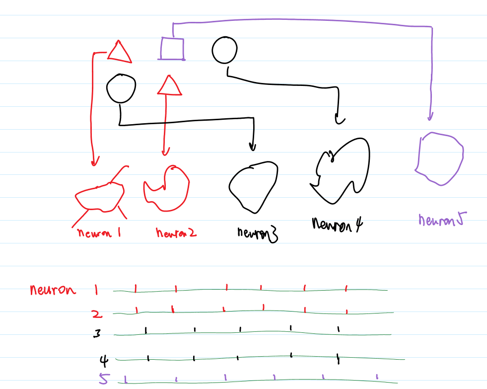
averaging over populations of neurons (fig 1.11) (another ensemble average):
- Population activity: $A(t) = \frac{\text{No. of spikes during time } t\sim t+\Delta t \text{ of all the }N \text{ neurons that has the same input}}{N}/\Delta t$
- No. of spikes during time $t\sim t+\Delta t$ of all the $N$ neurons that has the same input $n_{act}=\int_t^{t+\Delta}dt \text{ all spike written in delta function}=\int_t^{t+\Delta}dt \sum_j\sum_f \delta(t-t_j^{(f)})$.
- However,
- no actual homogeneous identical neurons
- Inhomogeneous? Population vector coding. $i$th neuron takes input $x_i$.
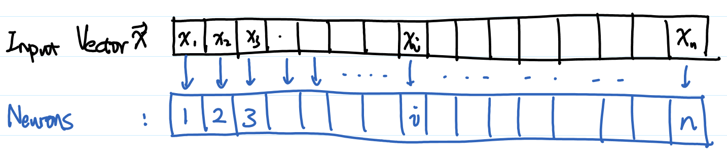
- Given a vector input, what is the average position (location on the vector index) of all neurons that gives output? $\mathrm{Average Location of Stimulated Neurons}=\frac{\int_t^{t+\Delta t} dt \sum_i \sum_f x_j \delta(t-t_j^{(f)}) }{\int_t^{t+\Delta t} dt \sum_i \sum_f \delta(t-t_j^{(f)}) }$.
- Used on neuronal activiy in primate motor cortex. <- Not sure how this is done.
Spike Codes
- Time-to-first-spike, a Simple Scheme of Spiking Codes: fig 1.12. Three neurons which are responsible for reading a picture of three pixels of three different color for example, will spike sequentially if each of them are responsible for a different color.
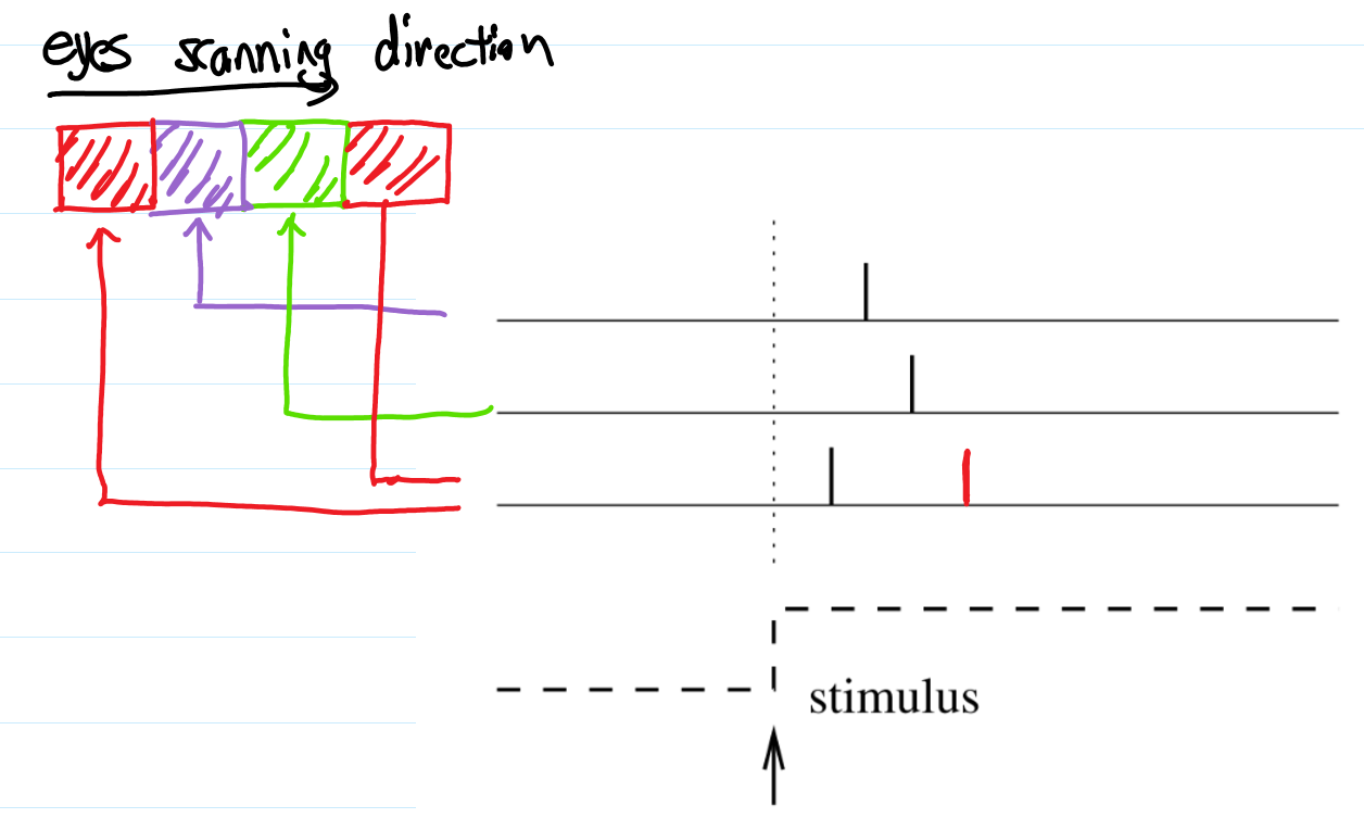
- Assuming each neuron is inactive after its spike <- due to some mysterious inhibition: this is called time-to-first-spike
- Coding by phase (fig 1.13): periodic spikes (common in hippocampus etc), relative phase between neurons (or relative to oscillatioins of background periodic spikes) could carry information.
- what is background oscillation? fig 1.14
- Example of sychronization and information
- Reverse correlation approach: investigate the averaged input instead of averaged PSTH (as we have done in Fig 1.10). So we find what input is required to generate a spike. Given spike train we can estimate the input by summing up the input of each spike! Fig 1.16B. Eqn 1.12.
Relation Between Spike Codes and Rate Codes
- Define a rate $\nu$ given a spike code, $\nu(t)=\frac{\text{effective number of spikes during time T}}{T}=\int d\tau K(\tau)S(t-\tau)/\int d\tau K(\tau)$, where $K(\tau)$ is window function which gives us the time interval of measurement, and $S(\tau)=\sum^n_{f=1}\delta(t-t^{(f)})$. So $\int d\tau K(\tau)S(t-\tau)$ is the number of spikes during the time window given by $K$.
- How to reconstruct rate code? If eqn 1.12 is true (linear reverse correlation approach is true) -> rate code, otherwise -> spike code.
- As an example, use Volterra expansion and drop the information about the reconstructed input correlations between two spikes.
Planted:
by KausalFlow;
References:
Dynamic Backlinks to
snm/limitations-srm-contd-and-coding: snm/limitations-srm-contd-and-coding Links to:
OctoMiao, OctoMiao Another Person (2016). 'Limitations of spike response model and coding', Connectome, 03 April. Available at: https://hugo-connectome.kausalflow.com/snm/limitations-srm-contd-and-coding/.